Description
Several data sets exist in datamuseum which have been
processed from their originally accessioned forms into digestible
formats to exemplify the workflow made possible by the package. These
are from the Global Biodiversity Information Facility (GBIF),
Invert-E-Base (InvBase), the Biological Information System for Marine
Life (BISMAL), Ocean Biodiversity Information System (OBIS), and one
data set obtained by direct request from the National Museum of Nature
and Science, Japan (NSMT).
The individual Japan-focused data sets can be found under Example Data at the Reference page.
Using the following packages:
Individual Data Sets
The raw and trimmed forms of each data set can be found on Github.
Global Biodiversity Information Facility (GBIF) Data
#Raw Data

GBIF_raw <- read.csv("GBIF_Octopodoidea_raw.csv") #88256 Observations

#Trimmed Data

GBIF_clean <- GBIF_raw[ -c(1:7, 11:15, 24:32, 34:36, 38, 40:50)]

GBIF_clean <- GBIF_clean[ -c(7, 9)] #88256 Observations

#Also available on Github as GBIF_Octopodoidea_trim.csv

#Japan Octopus Data

GBIF_Japan <- latlong_range(GBIF_clean, "decimalLatitude", "decimalLongitude",
                             25, 50, 125, 150, drop_na = TRUE) %>% dplyr::rename(
              "Prefecture" = "stateProvince",
              "Precise Location" = "locality", "Longitude" = "decimalLongitude", "Latitude" = "decimalLatitude",
              "Year" = "year", "Genus" = "genus", "Country" = "countryCode",
              "SciName" = "species", "Family" = "family","Source" = "institutionCode") #2145 Observations

GBIF_Japan <- replace(GBIF_Japan, GBIF_Japan=='', NA)

GBIF_Japan <- GBIF_Japan %>%
  filter(!is.na(Source) & !is.na(Family) &  !is.na(Genus) & !is.na(SciName)
         & !is.na(Year)) #798 Observations
The refined GBIF data, cleaned to Japan-adjacent waters and
superfamily Octopodoidea, can be found at: GBIF_Japan.
The GBIF_Japan data set was refined from the following occurrence download:
Global Biodiversity Information Facility (GBIF). GBIF.org (30 March 2026) GBIF Occurrence Download. https://www.gbif.org. doi: 10.15468/dl.2379hj
Invert-E-Base (InvBase) Data
#Raw Data

InvBase_raw <- read.csv("InvBase_Octopodoidea_raw.csv") #22608 Observations

#Trimmed Data

InvBase_clean <- InvBase_raw[ -c(1, 3:6, 8:13, 15:17, 19, 21:38, 40:62, 64:70, 72, 75:79, 82:103)] #22608 Observations

#Also available on Github as InvBase_Octopodoidea_trim.csv

#Japan Octopus Data

InvBase_Japan <- latlong_range(InvBase_clean, "decimalLatitude", "decimalLongitude",
                             25, 50, 125, 150, drop_na = TRUE) %>% dplyr::rename(
              "Prefecture" = "stateProvince", "Country" = "country",
              "Precise Location" = "county", "Longitude" = "decimalLongitude", "Latitude" = "decimalLatitude",
              "Year" = "year", "Genus" = "genus", "Source" = "institutionCode", "Family" = "family"
              ) #50 Observations

InvBase_Japan <- replace(InvBase_Japan, InvBase_Japan=='', NA)

InvBase_Japan <- InvBase_Japan %>%
  filter(!is.na(Source) & !is.na(Family) &  !is.na(Genus) & !is.na(specificEpithet)
         & !is.na(Year)) #43 Observations

taxon_column(InvBase_Japan, output = "list")

taxon_rank(InvBase_Japan, c(Family, Genus, specificEpithet))

InvBase_Japan <- taxon_combine(InvBase_Japan, genus = Genus, epithet = specificEpithet,
                            new_column = "SciName")

InvBase_Japan <- InvBase_Japan[ -c(5)]
The refined InvBase data, cleaned to Japan-adjacent waters and
superfamily Octopodoidea, can be found at: InvBase_Japan
Invert-E-Base. Downloaded 30 March 2026. https://invertebase.org
Biological Information System for Marine Life (BISMAL) Data
#Raw Data

BISMAL_raw <- read.csv("BISMAL_Octopodoidea_raw.csv") #1547 Observations

#Trimmed Data

BISMAL_clean <- BISMAL_raw[ -c(1:11, 13:18, 20:21, 23:49, 51:67, 67, 70,
                                       72:79, 82:99, 100:104, 106:108, 110, 112:116)] #1547 Observations

#Also available on Github as BISMAL_Octopodoidea_trim.csv

#Japan Octopus Data

BISMAL_Japan <- latlong_range(BISMAL_clean, "decimalLatitude", "decimalLongitude",
                             25, 50, 125, 150, drop_na = TRUE) %>% dplyr::rename( "Prefecture" = "stateProvince",
              "Precise Location" = "locality", "Longitude" = "decimalLongitude", "Latitude" = "decimalLatitude",
              "Year" = "year", "Genus" = "genus", "Country" = "country", "Source" = "institutionCode",
              "Family" = "family") #1507 Observations

BISMAL_Japan <- replace(BISMAL_Japan, BISMAL_Japan=='', NA)

BISMAL_Japan <- BISMAL_Japan %>%
  filter(!is.na(Source) & !is.na(Family) &  !is.na(Genus) & !is.na(specificEpithet)
         & !is.na(Year)) #473 Observations

taxon_column(BISMAL_Japan, output = "list")

taxon_rank(BISMAL_Japan, c(Family, Genus, specificEpithet))

BISMAL_Japan <- taxon_combine(BISMAL_Japan, genus = Genus, epithet = specificEpithet,
                            new_column = "SciName")

BISMAL_Japan <- BISMAL_Japan[ -c(12)]
The refined BISMAL data, cleaned to Japan-adjacent waters and
superfamily Octopodoidea, can be found at: BISMAL_Japan
Biological Information System for Marine Life (BISMAL). Downloaded 30 March 2026. https://www.godac.jamstec.go.jp/bismal/e/
Ocean Biodiversity Information System (OBIS)
#Raw Data

OBIS_raw <- read.csv("OBIS_Octopodoidea_raw.csv") #58526 Observations

#Trimmed Data

OBIS_clean <- OBIS_raw[ -c(0:20, 22:28, 30:39, 41, 44:63, 65:74, 76:100, 102:112, 114:127, 129:203, 205:209,
                                   211:282)] #58526 Observations

#Also available on Github as OBIS_Octopodoidea_trim.csv

#Japan Octopus Data

OBIS_Japan <- latlong_range(OBIS_clean, "decimalLatitude", "decimalLongitude",
                             25, 50, 125, 150, drop_na = TRUE) %>% dplyr::rename(
              "Prefecture" = "stateProvince", "Country" = "country",
              "Precise Location" = "locality", "Longitude" = "decimalLongitude", "Latitude" = "decimalLatitude",
              "Year" = "date_year", "Source" = "institutionCode", "Family" = "family", "Genus" = "genus",
              "SciName" = "species") #859 Observations

OBIS_Japan <- replace(OBIS_Japan, OBIS_Japan=='', NA)

OBIS_Japan <- OBIS_Japan %>%
  filter(!is.na(Source) & !is.na(Family) & !is.na(Genus) & !is.na(SciName)
         & !is.na(Year)) #698 Observations
The refined OBIS data, cleaned to Japan-adjacent waters and
superfamily Octopodoidea, can be found at: OBIS_Japan
Ocean Biodiversity Information System (OBIS). Downloaded 30 March 2026. https://obis.org
National Museum of Nature and Science, Japan (NSMT)
#Raw Data

NSMT_raw <- read.csv("NSMT_Octopodoidea_raw.csv") #870 Observations

#Trimmed Data

NSMT_clean <- NSMT_raw[ -c(5, 9:12, 16:18, 22:23)] #870 Observations

#Also available on Github as NSMT_Octopodoidea_trim.csv

#Japan Octopus Data

NSMT_Japan <- latlong_range(NSMT_clean, "Latitude", "Longitude",
                            25, 50, 125, 150, drop_na = TRUE) %>% dplyr::rename(
                              "Prefecture" = "Region", "Precise Location" = "Previse.loc.",
                              "Source" = "Group.Abb.") #727 Observations

NSMT_Japan <- replace(NSMT_Japan, NSMT_Japan=='', NA)

NSMT_Japan <- NSMT_Japan %>% filter(!is.na(Source) & !is.na(Family) & !is.na(Genus) &
                                      !is.na(Species)& !is.na(Year)) #726 Observations

taxon_column(NSMT_Japan, output = "list")

taxon_rank(NSMT_Japan, c(Family, Genus, Species))

NSMT_Japan <- taxon_combine(NSMT_Japan, genus = Genus, epithet = Species,
                            new_column = "SciName")

NSMT_Japan <- NSMT_Japan[ -c(6, 7)]
The refined NSMT data, cleaned to Japan-adjacent waters and
superfamily Octopodoidea, can be found at: NSMT_Japan
National Museum of Nature and Science, Japan (NSMT). Data obtained directly from the museum, early 2024. https://www.kahaku.go.jp/english/
Concatenated Data Sets
These data sets, made from combining the Japan-focused data, can be found under Example Data at the Reference page.
Japan Octopodoidea Data Set, museum
museum <- rbind(
  InvBase_Japan %>% mutate(`Data Frame` = "InvBase"),
  GBIF_Japan    %>% mutate(`Data Frame` = "GBIF"),
  NSMT_Japan   %>% mutate(`Data Frame` = "NSMT"),
  OBIS_Japan    %>% mutate(`Data Frame` = "OBIS"),
  BISMAL_Japan  %>% mutate(`Data Frame` = "BISMAL")
) #2738 Observations

museum <- deduplicate(museum, "catalogNumber",
                      drop_na = TRUE) #143 duplicate rows removed; 608 rows removed due to missing ID. 1987 Observations

museum_dupes <- attr(museum, "duplicates") #1268 Observations, 143 FALSE

museum <- duplicate(museum, "individualCount") #Duplication increased count from 1894 Observations to 2671 Observations
The concatenated Japanese Octopodoidea data, with repeat or absent
catalog numbers removed and specimen lots duplicated, can be found at:
museum
Japan Octopodoidea Data Set, museum_taxon
#Taxonomized Japan Octopus Data

museum_clean <- taxon_cleaner(museum, SciName, in_place = TRUE, drop_na = TRUE) #2260 Observations

museum_clean <- museum_clean %>% mutate(SciName = case_when(
    SciName == "Octopus vulgaris"        ~ "Octopus sinensis",
    TRUE                                 ~ SciName))

museum_valid <- taxon_validate(museum_clean, SciName, update_related = TRUE)

valid_report <- attr(museum_valid, "validation_report")

museum_check <- taxon_spellcheck(museum_valid, c(SciName), update = TRUE,
                                     validation_report = valid_report)

check_report <- attr(museum_check, "spellcheck_report")

museum_check <- museum_check %>%
  mutate(SciName = case_when(
    SciName == "Pinnoctopus macropus" ~ "Callistoctopus macropus",
    TRUE                              ~ SciName
  ))

museum_taxon <- taxon_add(museum_check, SciName, rank = c("order", "phylum", "family", "genus"),
                              author_year = FALSE, sort = FALSE)

add_report <- attr(museum_taxon, "add_report")

museum_taxon <-  museum_taxon[ -c(3,4)]

museum_taxon <- museum_taxon %>%
  dplyr::rename(
    "Order" = "order", "Phylum" = "phylum",
    "Family" = "family", "Genus" = "genus")

museum_taxon <- taxon_sort(museum_taxon)

museum_taxon <- taxon_cite(museum_taxon, c(Family, Genus, SciName))

cite_report <- attr(museum_taxon, "cite_report")

museum_taxon <- museum_taxon %>%
  filter(SciName != "Muusoctopus small in mature") %>%
  mutate(Family_cite = case_when(
    Family_cite == "Bathypolypodidae" ~ "Bathypolypodidae (G. C. Robson, 1929)",
    Family_cite == "Enteroctopodidae" ~ "Enteroctopodidae (Strugnell, M. Norman, Vecchione, Guzik & Allcock, 2014)",
    Family_cite == "Megaleledonidae" ~ "Megaleledonidae (Iw. Taki, 1961)",
    TRUE                              ~ Family_cite
  ))

museum_taxon <- italicize(museum_taxon, c(Genus_cite, SciName_cite))
The Japanese Octopodoidea data, with updates to its included
taxonomic data based on functions like taxon_validate(),
can be found at: museum_taxon
A map generated from museum_taxon
is shown below:
world_map <- map_data("world")

japan <- map_data("world", region="japan")

family_labels <- c(
  "Octopodidae (D'Orbigny, 1839-1842 in Férussac and D'Orbigny, 1834-1848)"   = "Octopodidae\n(D'Orbigny, 1839-1842\nin Férussac and\nD'Orbigny, 1834-1848)",
  "Amphitretidae (Hoyle, 1886)"                                                = "Amphitretidae\n(Hoyle, 1886)",
  "Enteroctopodidae (Strugnell, M. Norman, Vecchione, Guzik & Allcock, 2014)" = "Enteroctopodidae\n(Strugnell, M. Norman,\nVecchione, Guzik\n& Allcock, 2014)",
  "Bathypolypodidae (G. C. Robson, 1929)"                                             = "Bathypolypodidae\n(G. C. Robson, 1929)",
  "Megaleledonidae (Iw. Taki, 1961)"                                                  = "Megaleledonidae\n(Iw. Taki, 1961)"
)

lon_min <- 125
lon_max <- 150
lat_min <- 25
lat_max <- 50

museum_taxon$Longitude <- as.numeric(museum_taxon$Longitude)
museum_taxon$Latitude  <- as.numeric(museum_taxon$Latitude)

genera_per_family <- museum_taxon %>%
  select(Genus_cite_italic, Family) %>%
  distinct() %>%
  count(Family)

family_palettes <- list(
  "Amphitretidae"    = sequential_hcl(n = 2, palette = "BrwnYl",   l = c(30, 55)),
  "Bathypolypodidae" = sequential_hcl(n = 1, palette = "Reds",     l = c(45, 45)),
  "Enteroctopodidae" = sequential_hcl(n = 3, palette = "Peach"),
  "Megaleledonidae"  = sequential_hcl(n = 1, palette = "YlOrRd",   l = c(55, 55)),
  "Octopodidae"      = sequential_hcl(n = 7, palette = "Purples",  l = c(25, 65))
)

genus_family_map <- museum_taxon %>%
  select(Genus_cite_italic, Family) %>%
  distinct() %>%
  arrange(Family, Genus_cite_italic)  # arrange so shades are assigned alphabetically

genus_colors <- unlist(lapply(names(family_palettes), function(fam) {
  genera <- genus_family_map$Genus_cite_italic[genus_family_map$Family == fam]
  colors <- family_palettes[[fam]]
  setNames(colors, genera)
}))

# Create ordered breaks grouped by family
genus_order <- museum_taxon %>%
  select(Genus_cite_italic, Family, Family_cite) %>%
  distinct() %>%
  arrange(factor(Family, levels = c("Amphitretidae", "Bathypolypodidae",
                                     "Enteroctopodidae", "Megaleledonidae",
                                     "Octopodidae")),
          Genus_cite_italic)

# Step 1 - build genus_order_with_headers
genus_order_with_headers <- genus_order %>%
  group_by(Family) %>%
  group_modify(~ {
    family_cite_label <- paste0("bold(", .y$Family, ")")
    bind_rows(
      data.frame(
        Genus_cite_italic = family_cite_label,
        Family_cite       = .x$Family_cite[1]
      ),
      .x %>% select(Genus_cite_italic, Family_cite)
    )
  }) %>%
  ungroup() %>%
  pull(Genus_cite_italic)

# Step 2 - add spacer before Megaleledonidae
meg_pos <- which(genus_order_with_headers == "bold(Megaleledonidae)")
genus_order_with_headers <- c(
  genus_order_with_headers[1:(meg_pos - 1)],
  "' '",
  genus_order_with_headers[meg_pos:length(genus_order_with_headers)]
)

# Step 3 - build colors
header_colors <- setNames(
  rep("#FFFFFF00", 5),
  grep("^bold", genus_order_with_headers, value = TRUE)
)
spacer_color      <- setNames("#FFFFFF00", "' '")
genus_colors_final <- c(genus_colors, header_colors, spacer_color)

# Step 4 - legend overrides
legend_breaks <- intersect(genus_order_with_headers, names(genus_colors_final))
n <- length(legend_breaks)
spacer_pos <- which(legend_breaks == "' '")
header_pos <- which(grepl("^bold", legend_breaks))
hide_pos   <- c(spacer_pos, header_pos)

legend_size  <- ifelse(seq_along(legend_breaks) %in% hide_pos, 0, 8)
legend_alpha <- ifelse(seq_along(legend_breaks) %in% hide_pos, 0, 1)

legend_fill  <- rep(NA_character_, n)
legend_color <- rep(NA_character_, n)
legend_stroke <- rep(0.5, n)

legend_fill[hide_pos]   <- "transparent"
legend_color[hide_pos]  <- "transparent"
legend_stroke[hide_pos] <- 0

ggplot(data = world_map, aes(long, lat)) +
  geom_polygon(aes(group = group)) +
  coord_sf(xlim   = c(lon_min - 1, lon_max + 1), ylim   = c(lat_min - 1, lat_max + 1),
  expand = FALSE) +
  geom_point(data = museum_taxon,
             aes(x = Longitude, y = Latitude, color = Genus_cite_italic),
             size = 3,
             position = position_jitter(width = .1, height = .1)) +
  labs(x = "Longitude", y = "Latitude", color = "Genus") +
  scale_colour_manual(
  values = genus_colors_final,
  breaks = genus_order_with_headers,
  limits = names(genus_colors_final),
  labels = function(x) lapply(x, function(i) parse(text = i))
  ) +
  guides(
  color = guide_legend(
    override.aes = list(
      size  = legend_size,
      alpha = legend_alpha), ncol = 4
  )) +
  theme(
  plot.margin        = margin(t = .05, r = 1, b = .05, l = 1, unit = "mm"),
  legend.key         = element_rect(fill = "transparent", color = "transparent"),
  legend.position        = "bottom",
  legend.title.position  = "top",
  legend.spacing.y   = unit(0.25, "mm"),
  legend.spacing.x   = unit(1, "mm"),
  legend.title           = element_text(size = 16),
  legend.text            = element_text(size = 14),
  strip.text             = element_text(size = 16),
  axis.title             = element_text(size = 20),
  axis.text.x            = element_text(size = 16, angle = 60, hjust = 1),
  axis.text.y            = element_text(size = 16)
) +
  facet_wrap(~Family_cite, nrow = 1, labeller = as_labeller(family_labels))

ggsave("octopodoidea_japan.png", width = 16, height = 7.5, units = "in", dpi = 450)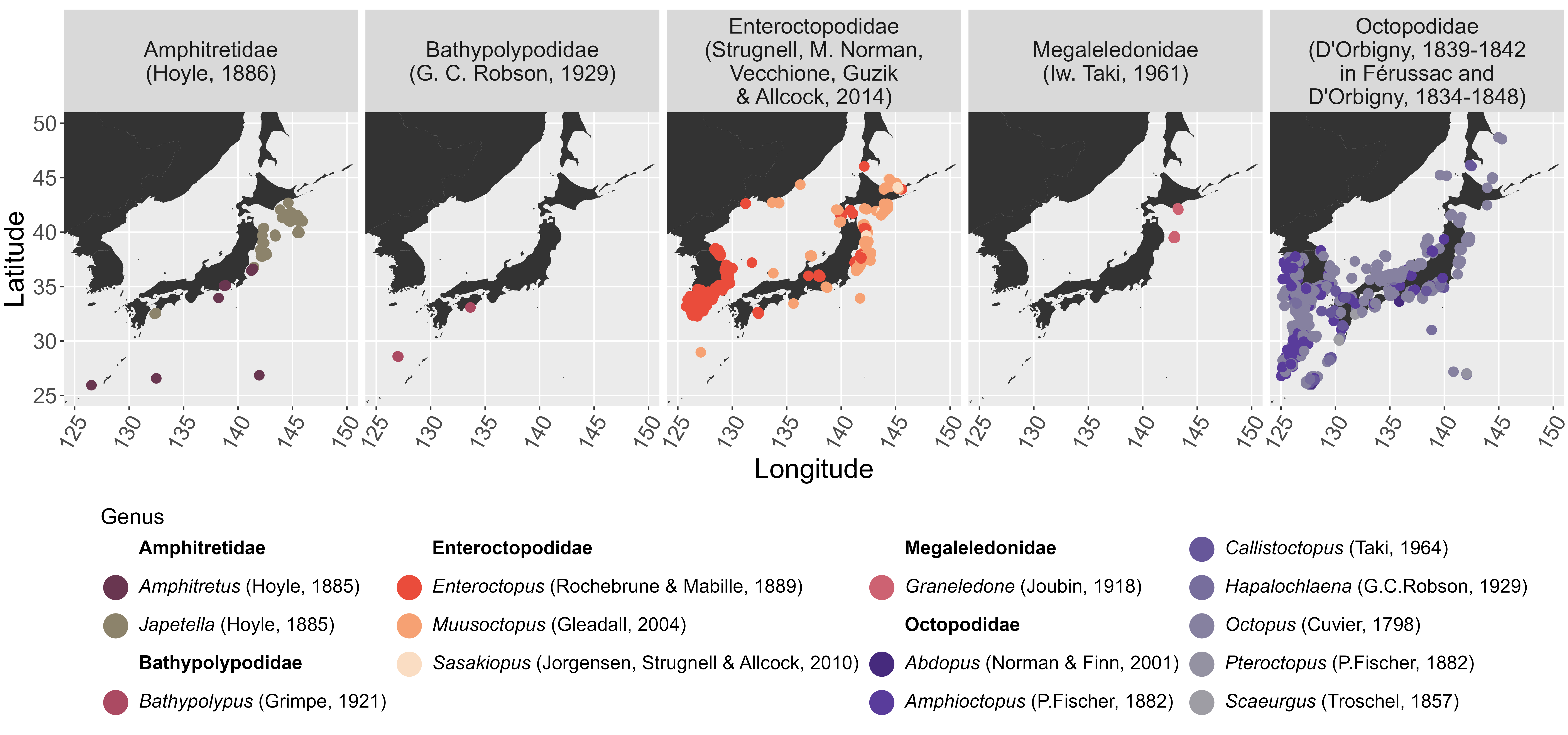
Octopodoidea occurrences in Japan by family and genus.